plot.species_mix_effects_data
Arguments
- x
a list of partial prediction data frames as generated by effects_data
- object
A fitted species_mix model.
- boot.object
A species_mix.bootsrap object. Default is NULL, no standard errors will be reported.
- nboot
An option to do bootstrapping when plotting, this will be slow, better to run and save bootstrap object and pass to plotting function as boot.object.
- type
The type of prediction. Default is 'response' alternative is 'link'.
- response.var
What response variable to plot on the y-axis. Default is all Archetypes. Other options are a subset of Archetypes, names "Archetype1". Or species can be plotted, "Species" will plot all species predictions in the model. "SpeciesSum" with sum all species predictions on the y-axis, for a binomial model this will represent species richness. For other models, it will be the sum of the species specific responses. Finally, individual species can be plotted using the species name in the original response data.
- CI
is the confidence intervals for the stand errors.
- linecols
Are the default colours for plotting the partial responses.
- polycols
Is the colour of the confidence intervals in the response plots.
- ylim
Default is NULL and will plot ylim within range of the response variable.
- \dots
Extra plotting arguments.
Details
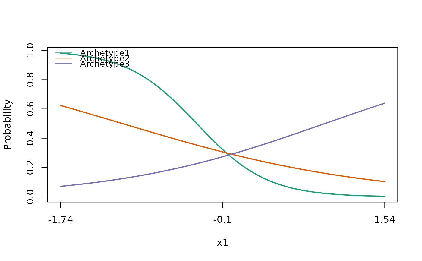
Plots the partial dependence plots (marginal response curves) for focal covariates. Continuous covariates will be plotted as lines, factors will be plotted as dotplots.
Examples
# \donttest{
library(ecomix)
set.seed(42)
sam_form <- stats::as.formula(paste0('cbind(',paste(paste0('spp',1:20),
collapse = ','),")~x1+z1"))
sp_form <- ~ 1
beta <- matrix(c(-2.9,-3.6,-0.9,1,.9,1.9),3,2,byrow=TRUE)
dat <- data.frame(y=rep(1,100),x1=stats::runif(100,0,2.5),
z1=stats::rnorm(100,0,2.5))
dat[,-1] <- scale(dat[,-1])
simulated_data <- species_mix.simulate(archetype_formula = sam_form,species_formula = sp_form,
data = dat,beta=beta,family="bernoulli")
#> Random alpha from normal (-1,0.5) distribution
fm1 <- species_mix(archetype_formula = sam_form,species_formula = sp_form,
data = simulated_data, family = 'bernoulli', nArchetypes=3)
#> SAM modelling
#> There are 3 archetypes
#> There are 100 site observations for 20 species
#> The model for the archetype (grouping) is ~x1 + z1
#> The model for the species is ~1
#> You are implementing a bernoulli Species Archetype Model.
#> This model uses a logit link function.
#> Using ECM algorithm to find starting values; using 1 refits
#> ECM restart 1 of 1
#> Initialising starting values
#> Initial groups parameter estimates by K-means clustering
#> Iteration: 1 | New loglik -950.728 | Ratio loglik 0
#> Iteration: 2 | New loglik -829.843 | Ratio loglik 0.8728
#> Iteration: 3 | New loglik -820.246 | Ratio loglik 0.9884
#> Iteration: 4 | New loglik -819.839 | Ratio loglik 0.9995
#> initial value 819.837517
#> iter 10 value 819.706573
#> final value 819.703416
#> converged
eff.df <- effects_data("x1",fm1)
plot(eff.df,fm1)
 # }
# }