Species Archetype Models
The Species Archetype Models (SAMs) are variant of ‘Mixture-of-Regressions’ and try to describe how homogeneous groups of species vary with the environment. These groups are referred to as Species Archetypes (Dunstan et al. 2011). Each Archetype represents a group of species which jointly response to environmental data in the model (covariates). For example, one group of species might like warm water, while another might like cold. Typically, we model observations of species at sites. The covariates are used to describe the variation (and response) of each Archetype to the physical and environmental gradients. We can describe the data as \(i = 1...n\) sampling sites, \(j = 1...S\) species (or desired taxonomic unit) and \(k = 1...K\) Archetypes. The model conditional mean observations (occurrence/count/biomass) of species is, \(\mathbb{E}(y_{ij}|\textrm{archetype group_k})\), on \(g_k(X_i)\) Archetype covariates. In ecomix, the intercepts are species-specific, this is an update from the original ‘SpeciesMix’ R package (Dunstan et al. 2013a), where the intercepts were only species-specific for the Negative Binomial and Tweedie distributions, as described in Dunstan et al. (2013b). For error distributions with dispersion or variance parameters (Negative Binomial, Tweedie and Gaussian) these parameters are also species-specific. The model can be described as follows:
\[ \begin{equation} h[\mathbb{E}(y_{ij}|\phi_{k})] = \alpha_j + g_k(X_{i}^\top\beta_{k}) + \nu_i \tag{1}\label{eq:one} \end{equation} \]
where \(Pr(\phi_{k}) = \pi_k,\) and \(\sum^K_{k=1}{\pi_k=1}\). The functional form of \(g_k(.)\) can be specified to be any function commonly used within a Generalized Linear Model framework. Including linear, quadratic, spline and interaction terms. Additionally an offset term \(\nu_i\) can be included to account for sampling artefacts and are included into the model on a log-scale (e.g. log(area sampled)). We refer to the model as the species_mix in the ecomix package.
Here we will demonstrate how to fit and interpret a Species Archetype Models (SAMs) from our ecomix package. We will present a simulation study to demonstrate the functionality of species_mix.
Simulate Environmental Data
We generate a set of simulated environment predictors using Gaussian random fields with nugget effects on some of the variables.
library(raster)
library(RandomFields)
set.seed(007)
lenny <- 100
xSeq <- seq( from=0, to=1, length=lenny)
ySeq <- seq( from=0, to=1, length=lenny)
X <- expand.grid( x=xSeq, y=ySeq)
Mod1 <- RMgauss( var=1, scale=0.2) + RMnugget( var=0.01)
Mod2 <- RMgauss( var=1, scale=0.5) + RMnugget( var=0.01)
Mod3 <- RMgauss( var=1, scale=1)# + RMnugget( var=0.01)
Mod4 <- RMgauss( var=2, scale=0.1) + RMnugget( var=1)
simmy1 <- RFsimulate( Mod1, x=xSeq, y=ySeq)
simmy2 <- RFsimulate( Mod2, x=xSeq, y=ySeq)
simmy3 <- RFsimulate( Mod3, x=xSeq, y=ySeq)
simmy4 <- RFsimulate( Mod4, x=xSeq, y=ySeq)
X <- cbind( X, as.numeric( as.matrix( simmy1)), as.numeric( as.matrix( simmy2)),
            as.numeric( as.matrix( simmy3)), as.numeric( as.matrix( simmy4)))
X[,-(1:2)] <- apply( X[,-(1:2)], 2, scale)
colnames( X) <- c("x","y","covar1","covar2","covar3","covar4")
env <- rasterFromXYZ( X)
names(env) <- c("Temperature", "Oxygen", "Depth", "Productivity")
env.df <- as.data.frame(env,xy=TRUE)
env_dat<-rasterToPoints(env)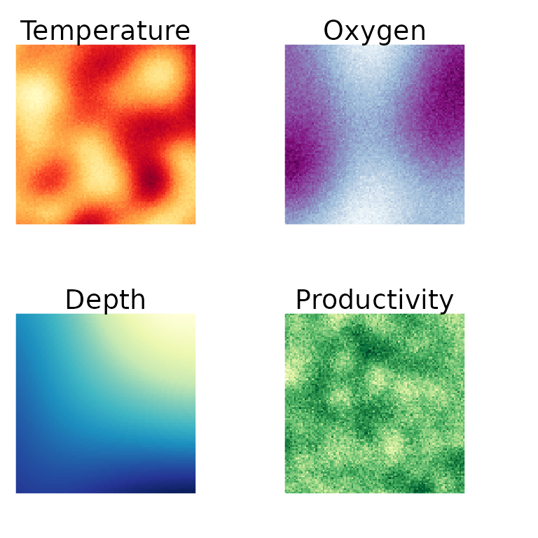
Figure 1. Simulated environmental variables used in Species Archetype Modelling
Simulate Biological Data
We simulated a set of synthetic species to be fitted using the species_mix function. We generated the expected species intercepts \(\alpha_j\) from a beta distribution, and assign known group level covariates \(\beta_k\). \(\beta_k\) represents the archetype (group) response to each covariate in the model. We simulated species archetypical responses using the species_mix.simulate function. If no known parameters are provided random parameters will be generated for the formula and data provided. Here we provided parameters for the species intercepts (alphas) and the archetype mean responses (betas).
set.seed(42)
nsp <- 100
betamean <- 0.3
betabeta <- 2
betaalpha <- betamean/(1-betamean)
alpha <- rbeta( nsp, betaalpha, betabeta)
alphas <- log( alpha / ( 1-alpha))

betas <- as.matrix(data.frame(Temperature=c(0.75,0,1.5),
                              Temperature2=c(-0.75,0,0),
                              Oxygen=c(0,0.5,0),
                              Oxygen2=c(0,-0.5,0),
                              Depth= c(-1.5,0.5,1.5),
                              Depth2= c(0,-0.5,0),
                              Productivity=c(1,0,-2.5),
                              Productivity2=c(-1,0,0),
                              Time=rnorm(3)))
rownames(betas) <- paste0("Archetype.",1:3)

# generate realisation of data for entire survey region
sim_dat <- data.frame(intercept=1,env_dat[,3:ncol(env_dat)])
sites<-sample(1:nrow(sim_dat), 200, replace=FALSE)
env_200<-sim_dat[sites,]
env_200$Time <- sample(c(0,1),size = 200, replace = TRUE)

sam_form <- stats::as.formula(paste0('cbind(',paste(paste0('spp',1:100),
collapse = ','),")~poly(Temperature,degree=2,raw=TRUE)+poly(Oxygen,degree=2,raw=TRUE)+poly(Depth,degree=2,raw=TRUE)+poly(Productivity,degree=2,raw=TRUE)+Time"))
sp_form <- ~1
simulated_data200 <- species_mix.simulate(archetype_formula=sam_form,
                                       species_formula=sp_form,
                                       alpha = alphas,
                                       beta = betas,
                                       data = env_200,
                                       nArchetypes = 3,
                                       family = "bernoulli")
Model fitting and evaluation
We have generated occurrence records for 100 synthetic species across the 200 randomly surveyed sites. Because we have presence and absence data we can fit a SAM with a Bernoulli family. In this example, we may chose to remove the rare species (< 10 occurrences across all sites). These species could be potentially included in the model, but would likely create noise and unexplained variance, making the model harder to fit and estimate (Hui et al. 2013).
count <- table(colSums(simulated_data200[,1:100]))
occur <- as.numeric(names(count))
mat <- as.data.frame(cbind(occur,count))
df1 <- merge(data.frame(occur = 0:max(mat[,1])), mat, all.x=TRUE)
df1$count[is.na(df1$count)] <- 0
bp <- barplot(count~occur, data= df1, xaxt='n', ylab="Count of Species",xlab="Number of Species's Occurrences")
abline(v=10,col='red',lwd=2)
bpdf <- cbind(bp,df1)
axis(1, at=bp[c(0,25,50,75,100,nrow(bpdf)-1)+1,1], labels = c(0,25,50,75,100,""),las=1)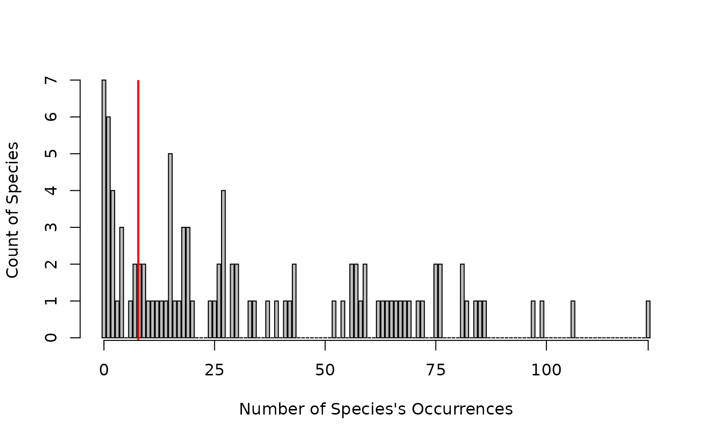
Figure 2. The simulated occurrences for the 100 species. We will remove all species with less than 10 presences across all 200 sites.
In this, example we fit independent polynomials with two degrees of freedom for the four simulated covariates Temperature, Oxygen, Depth & Productivity. We do this to demonstrate a simple simulated example where can show the known response of covariates to simulated data. We include time as a factor, which represents the time in which the simulated samples were recorded, for these data the two factors are ‘Day’ or ‘Night’. But additional discrete times could be included such as years. Below is a small code block with a basic example on how to fit a single species_mix model.
## load the ecomix package
library(ecomix)

## Select species with greater than ten occurrences across all sites.
spdata <- simulated_data200[,1:100]
spdata <- spdata[,-which(colSums(simulated_data200[,1:100])<10)]
samdat_10p <- cbind(spdata,env_200)
samdat_10p$Time <- as.factor(ifelse(samdat_10p$Time>0,"Night","Day"))

## Archetype formula
archetype_formula <- as.formula(paste0(paste0('cbind(',paste(colnames(samdat_10p)[grep("spp",colnames(samdat_10p))],collapse = ", "),") ~ poly(Temperature,degree=2,raw=TRUE)+poly(Oxygen,degree=2,raw=TRUE)+poly(Depth,degree=2,raw=TRUE)+poly(Productivity,degree=2,raw=TRUE)+Time")))

## Species formula
species_formula <- ~ 1

## Fit a single model
sam_fit <- species_mix(archetype_formula = archetype_formula, # Archetype formula
                       species_formula = species_formula,    # Species formula
                       data = samdat_10p,            # Data
                       nArchetypes = 3,              # Number of groups (mixtures) to fit
                       family = 'bernoulli',         # Which family to use
                       control = list(quiet = TRUE))
Group selection
One challenge when developing SAMs (or any finite mixture model) is selecting \(k\); the number of groups (archetypes) in the model. The number of archetypes is latent, so must be estimated from the data and the functional form of the covariates. In this example, we know that the optimal number of groups for these data is three, because we simulated the data with these characteristics. However, \(k\) is generally not known in real world applications. So one import part of the fitting process is finding \(k\), having said that it is also totally fine to define \(k\) for say a management objective. We can estimate the “best” number of groups based on the most parsimonious fit to the data. We can do this based on the model log-likelihood, and information criterion such as BIC. We provide a function species_mix.multifit which can assist in group selection if a vector of archetypes is provided. Below is an example of how one might do this. For simplicity we have left the nstart=1, but for more complex models this could be increased to use multiple starts to help search to the likelihood.
nArchetypes <- 1:6
sam_multifit <- species_mix.multifit(archetype_formula = archetype_formula, # Archetype formula
                                     species_formula = species_formula,     # Species formula
                                     data = samdat_10p,                     # Data
                                     nArchetypes = nArchetypes,             # Number of groups (mixtures) to fit
                                     nstart = 1,                            # The number of fits per archetype.
                                     family = 'bernoulli',                  # Which family to use
                                     control = list(quiet = FALSE))
plot(sam_multifit,type="BIC")
Model diagnostics and checking
Once we selected the ‘best’ model we can start to explore the model fit via diagnostics and checks. Typically, we would look at the model residuals to understand the model diagnostics (Warton et al. 2015). Here we present the random quantile residuals (Dunn & Smyth 1996) versus the fitted values from the model. We can see the residuals, presented on a species by species level, are approximately randomly distributed along the fitted line, which suggests nothing is untoward with the model fit.
plot(sam_fit,fitted.scale = 'logit')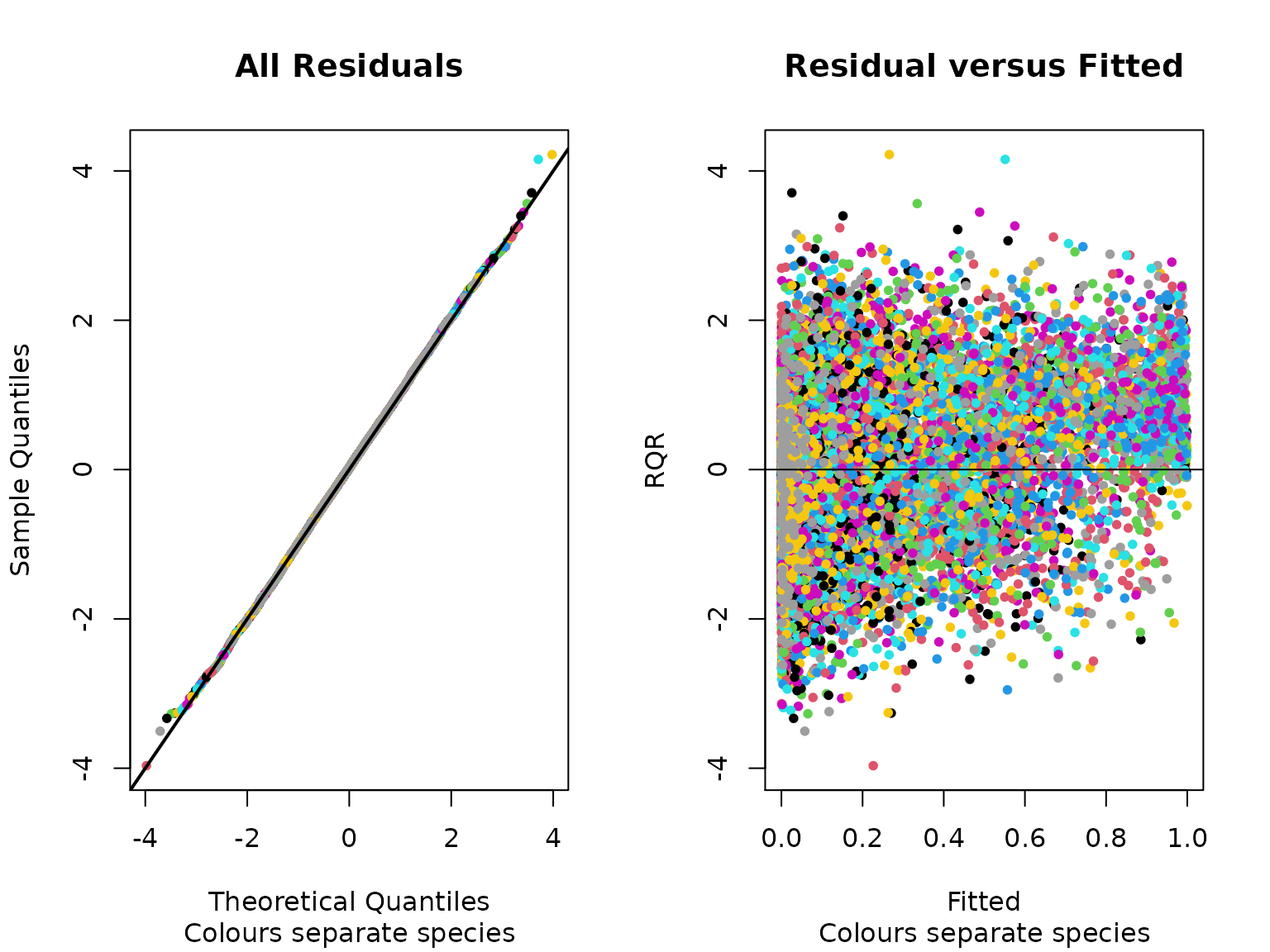
Figure 4. Random quantile residuals for all species in the fitted model.
We can also look at the random quantile residuals for a single species
plot(sam_fit,fitted.scale = 'logit', species="spp3")
Figure 5. Random quantile residuals for spp3 from the fitted model.
We can also plot the partial responses of covariates as shown in Dunstan et al. (2011) & Hui et al. (2013). The idea behind this approach is to understand the response of archetypes to a focal predictor. Firstly, we need to set up a data.frame which allows the focal.predictor to vary and averages over the other effects in the model. We demonstrate how to this in the next code chunk. We can include estimates of uncertainty in the partial response plots by including a bootstrap object into the plot function, otherwise the mean response is plotted without uncertainty in the partial response.
par(mfrow=c(2,3))
eff.df <- effectPlotData(focal.predictors = c("Temperature","Oxygen","Productivity","Depth","Time"), sam_fit)
sam_boot <- species_mix.bootstrap(sam_fit,nboot = 10, quiet = TRUE)
#> ..........
plot(x = eff.df, object = sam_fit, object2=sam_boot,ylim=c(0,1))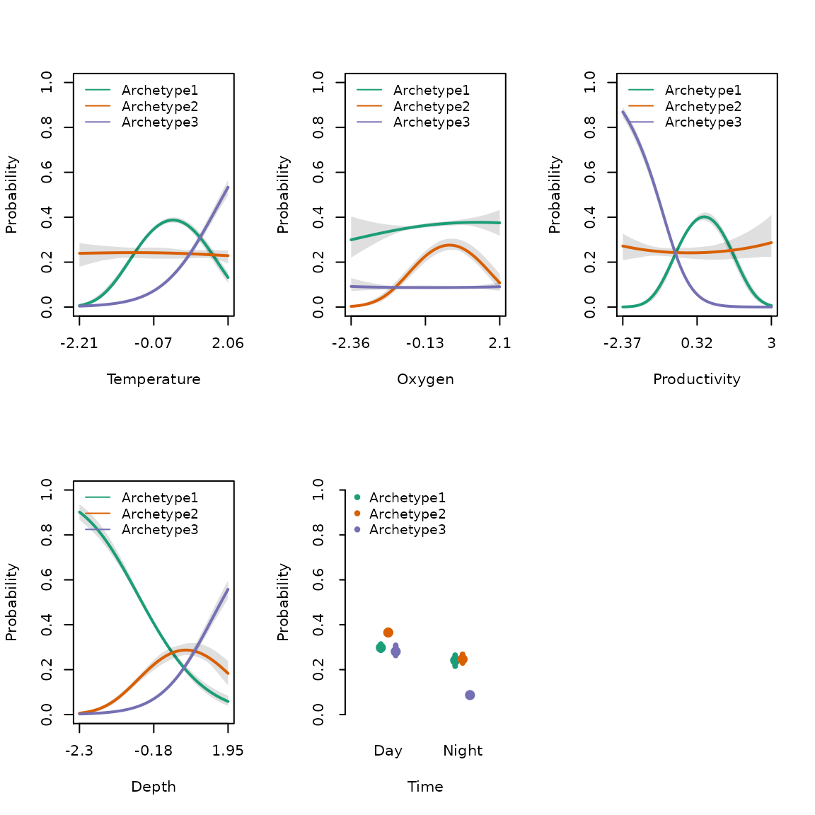
Figure 6. Partial response plots for each covariate in the model.
Model prediction
We can generate predictions for the each archetype in ecomix using predict() function. The default is used to generate a point mean estimate for each archetype. With the inclusion of a species_mix.bootstrap object we can also provide estimates of uncertainty or standard error for each prediction. We can see spatial predict the point mean and standard error in the predicted distributions of each archetype (Fig. 3e & 3f). We can also see the spatial response of each archetype is strongly correlated to it’s environmental response to each covariate (Fig. 2). For example, archetype two has a strong response to depth (Fig. 3e), which is evident in the archetype responses (Fig. 3d).
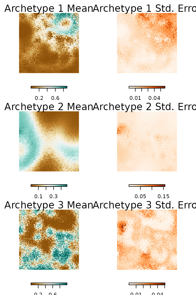
Figure 7. The predicted probability of each species archetype across the simulated environment and the standard error of the predictions generated based on the Bayesian bootstrap.